.ipynb .pdf

Contents

Model Training Tutorial

Welcome to the model training tutorial! In this tutorial, we will train a neural network to classify tiles from our toy data set and visualize its efficacy. For now, the classifier code in full can be found at: https://github.com/msk-mind/sandbox/blob/master/classifier/crc_tile_classifier/tile_classifier.py. Our model is essentially a wrapper around PyTorch’s ResNet 18 deep residual network; the LUNA team modified it to suit their work with tiling the slides. Here are the steps we will review in this notebook:

• Initialize project space for model

• Import libraries and set constants

• Define parameters and set output directory

• Load and prepare data

• Define model

• Train and save model

• Visualize TensorBoard logging

Initialize project space for model

First, you must initialize a directory for the model and its outputs.

%%bash

mkdir PRO_12-123/model/
mkdir PRO_12-123/model/outputs

Import libraries and set constants

Since we are not using CLIs with built-in import statements for this notebook, it is necessary to include this on our own.

# todo: remove libs
import datetime
import sys
import os

from collections import Counter
from typing import List, Optional, Tuple

sys.path.append(os.pardir)

import matplotlib.pyplot as plt
import pickle
import numpy as np
import pandas as pd
import pyarrow.dataset as ds
import pyarrow.parquet as pq

import torch

import torch.nn as nn
import torch.optim as optim
import torchvision.models as models

from PIL import Image
from pyarrow import fs
from tensorboard import notebook
from torchvision import transforms
from torch.utils.data import Dataset, DataLoader
from torch.utils.data.sampler import SubsetRandomSampler

from classifier.model import Classifier
from classifier.data import (
    TileDataset,
    get_stratified_sampler,
    get_group_stratified_sampler,
)
from classifier.utils import set_seed, seed_workers

# constants
torch.set_default_tensor_type(torch.FloatTensor)

Define parameters and set output directories

Next, you will define parameters that are crucial to your model. You will also Here are some notes to explain the parameters:

• batch_size refers to the number of training examples used in one iteration (number of times the algorithm’s parameters are updated); this model runs with mini-batch mode, where the batch size is less than the total dataset size but greater than one.

• validation_split refers to the percentage of data that will be used to validate the efficacy of the model as opposed to data that will be used to train the model.

• shuffle_dataset is set to true in order for the model to randomize the order of samples within batches between epochs

• random_seed is the starting point for generating random numbers in a number sequence. Randomness will be used in many different aspects of the machine learning algorithm, such as shuffling the datset between epochs and randomly initializing weights for the parameters.

• lr refers to the learning rate of the gradient descent optimizer.

• epochs refers to the number of times the algorithm will loop through the entire dataset during training. Setting this variable to 10 specifies that the dataset will be run through 10 times before the model is finished training.

# define params
batch_size = 64
validation_split = 0.50
shuffle_dataset = False
random_seed = 42
lr = 1e-3
epochs = 10
n_workers = 20

# set random seed
set_seed(random_seed)

You will also set your output directory. This directory will include the checkpoints from the model as well as outputs that will enable the TensorBoard extension to generate figures documenting the model’s progression as it trains on the data.

# set output directory
output_dir = 'PRO_12-123/model/outputs/'

Load and prepare data

First, we must specify attributes of our data: the label set and path. The regional annotations referenced many properties of each image, and we will train our model on five of the most prevalent properties. Note that the tumor class must correspond to the first label in the label set; otherwise, our inference will be incorrect further down the pipeline.

# load data
label_set = {
    "tumor":0,
    "vessels":1,
    "stroma":2
}

We must also specify the path to our data and load it into a pandas dataframe. We may see the labels present in our data and the number of instances in each data by taking a closer look at the dataframe.

path_to_tile_manifest = 'PRO_12-123/tiles/ov_tileset'
df = pq.ParquetDataset(path_to_tile_manifest).read().to_pandas()

print(df.groupby("regional_label").size())

regional_label
adipocytes              45
arteries              3921
lympho_poor_tumor     3806
lympho_rich_stroma     991
lympho_rich_tumor     5739
veins                  194
dtype: int64

To make classification simpler and more effective, we will do additional processing of the data. Specifically, we will group together lympho_poor_tumor and lympho_rich tumor under a generic tumor class, link arteries and veins under a vessels class, as well as remove classes with relatively few samples to get rid of noise. After doing so, we may check the regional labels again. Note that the tumor classes grew in size and that there are fewer labels in total. Our regional labels now match the label_set that we defined earlier.

df['regional_label'] = df['regional_label'].str.replace('arteries', 'vessels')
df['regional_label'] = df['regional_label'].str.replace('veins', 'vessels')

df['regional_label'] = df['regional_label'].str.replace('lympho_poor_tumor', 'tumor')
df['regional_label'] = df['regional_label'].str.replace('lympho_rich_tumor', 'tumor')

df['regional_label'] = df['regional_label'].str.replace('lympho_rich_stroma', 'stroma')

df = df[df['regional_label'] != 'adipocytes']

print(df.groupby("regional_label").size())

regional_label
stroma      991
tumor      9545
vessels    4115
dtype: int64

TileDataset is a class that inherits from the PyTorch Dataset class. It transforms our dataset into a Tensor, specifies the labelset, and defines functions to calculate the length of the dataset and to get an item from the dataset. The main difference between this class and the PyTorch class is the latter function; to retrieve an item from the dataset, TileDataset uses image offset to retrieve a tile from an image.

dataset_local = TileDataset(df, label_set)

With just a little more processing, we can reset the indices in our dataframe, convert patient IDs to numerical values if need be (in this case, our patient IDs are already numeric, so this line is commented out), and convert regional labels to integers.

# reset index
df_nh = df.reset_index()
# convert patient_ids to numerical values
# df_nh['patient_id'] = [id[2:] for id in df_nh['patient_id']]
# convert labels to ints
df_nh['regional_label'] = [label_set[label] for label in df_nh['regional_label']]
df_nh

	patient_id	id_slide_container	address	coordinates	otsu_score	purple_score	regional_label	tile_image_offset	tile_image_length	tile_image_size_xy	tile_image_mode	data_path
0	4	2551028	x128_y72_z20	(128, 72)	1.0	1.0	1	4.446781e+08	49152.0	128.0	RGB	/gpfs/mskmindhdp_emc/user/shared_data_folder/p...
1	4	2551028	x128_y73_z20	(128, 73)	1.0	1.0	1	4.447273e+08	49152.0	128.0	RGB	/gpfs/mskmindhdp_emc/user/shared_data_folder/p...
2	4	2551028	x128_y74_z20	(128, 74)	1.0	1.0	1	4.447764e+08	49152.0	128.0	RGB	/gpfs/mskmindhdp_emc/user/shared_data_folder/p...
3	4	2551028	x128_y75_z20	(128, 75)	1.0	1.0	1	4.448256e+08	49152.0	128.0	RGB	/gpfs/mskmindhdp_emc/user/shared_data_folder/p...
4	4	2551028	x128_y76_z20	(128, 76)	1.0	1.0	1	4.448748e+08	49152.0	128.0	RGB	/gpfs/mskmindhdp_emc/user/shared_data_folder/p...
...	...	...	...	...	...	...	...	...	...	...	...	...
14646	1	2551571	x453_y148_z20	(453, 148)	1.0	1.0	0	3.706257e+09	49152.0	128.0	RGB	/gpfs/mskmindhdp_emc/user/shared_data_folder/p...
14647	1	2551571	x454_y146_z20	(454, 146)	1.0	1.0	0	3.713237e+09	49152.0	128.0	RGB	/gpfs/mskmindhdp_emc/user/shared_data_folder/p...
14648	1	2551571	x454_y147_z20	(454, 147)	1.0	1.0	0	3.713286e+09	49152.0	128.0	RGB	/gpfs/mskmindhdp_emc/user/shared_data_folder/p...
14649	1	2551571	x454_y148_z20	(454, 148)	1.0	1.0	0	3.713335e+09	49152.0	128.0	RGB	/gpfs/mskmindhdp_emc/user/shared_data_folder/p...
14650	1	2551571	x455_y143_z20	(455, 143)	1.0	1.0	2	3.719725e+09	49152.0	128.0	RGB	/gpfs/mskmindhdp_emc/user/shared_data_folder/p...

14651 rows × 12 columns

Our model would have biased predictions if data from the same patient appeared in both the training and the validation set. This is because the model would be validating on near-identical data to data it has already seen.

Additionally, in order to maximize the efficacy of our model, it is important to protect against an unbalanced amount of data from each label set appearing in the test and validation sets. For instance, if our model was trained on mostly tumor and arteries data (data with many instances in the dataset), then it might incorrectly identify data labeled as a vein if it saw that data in the validation set.

For these two reasons, it is critical to stratisfy our data by patient ID while balancing regional labels. We pass our data through a function to do this.

# stratify by patient id while balancing regional_label
train_sampler, val_sampler = get_group_stratified_sampler(
    df_nh, df_nh["regional_label"], df_nh["patient_id"], split=validation_split
)
print(next(iter(train_sampler)))
print(next(iter(val_sampler)))

10804
2125

train_loader = DataLoader(
        dataset_local,
        num_workers=n_workers,
        worker_init_fn=seed_workers,
        shuffle=shuffle_dataset,
        batch_size=batch_size,
        sampler=train_sampler,
    )

validation_loader = DataLoader(
        dataset_local,
        num_workers=n_workers,
        worker_init_fn=seed_workers,
        shuffle=shuffle_dataset,
        batch_size=batch_size,
        sampler=val_sampler,
    )

data = {"train": train_loader, "val": validation_loader}
print(len(train_loader))
print(len(validation_loader))

127
103

Next, we will define the model. This model uses a ResNet18 architecture built into PyTorch, a commonly used deep residual network, and optimized the Adam gradient descent optimizer

# define model
network = models.resnet18(num_classes=len(label_set))
optimizer = optim.Adam(network.parameters(), lr=lr)

# class balanced cross entropy
train_labels = df_nh["regional_label"][train_sampler]
#class_weights = torch.Tensor([1/count for count in Counter(train_labels).values()])

#criterion = nn.CrossEntropyLoss(weight = class_weights.to(device='cuda'))
criterion = nn.CrossEntropyLoss()

Train and save model

Finally, we are ready to train our classifier and save it in the output file!

%%time

model = Classifier(
        network,
        criterion,
        optimizer,
        data,
        label_set,
        output_dir=output_dir,
    )

for n_epoch in range(epochs):
    print(n_epoch)
    _ = model.train(n_epoch)

    if n_epoch % 2 == 0:
        print("validating")
        _ = model.validate(n_epoch)
        model.save_ckpt(os.path.join(output_dir, 'ckpts'))

pass

0
validating

/gpfs/mskmindhdp_emc/user/shared_data_folder/pathology-tutorial/classifier/analyze.py:30: RuntimeWarning: invalid value encountered in true_divide
  cm_perc = cm / cm_sum.astype(float) * 100

saved model checkpoint
1
2
validating

/gpfs/mskmindhdp_emc/user/shared_data_folder/pathology-tutorial/classifier/analyze.py:30: RuntimeWarning: invalid value encountered in true_divide
  cm_perc = cm / cm_sum.astype(float) * 100

saved model checkpoint
3
4
validating

/gpfs/mskmindhdp_emc/user/shared_data_folder/pathology-tutorial/classifier/analyze.py:30: RuntimeWarning: invalid value encountered in true_divide
  cm_perc = cm / cm_sum.astype(float) * 100

saved model checkpoint
5
6
validating

/gpfs/mskmindhdp_emc/user/shared_data_folder/pathology-tutorial/classifier/analyze.py:30: RuntimeWarning: invalid value encountered in true_divide
  cm_perc = cm / cm_sum.astype(float) * 100

saved model checkpoint
7
8
validating

/gpfs/mskmindhdp_emc/user/shared_data_folder/pathology-tutorial/classifier/analyze.py:30: RuntimeWarning: invalid value encountered in true_divide
  cm_perc = cm / cm_sum.astype(float) * 100

saved model checkpoint
9
CPU times: user 2min 25s, sys: 1min 38s, total: 4min 3s
Wall time: 5min 9s

Visualize TensorBoard logging

Tensorboard is a tool used to inspect and understand machine learning models. We will use it to provide measurements for our model and view the outputs. First, we must load the TensorBoard notebook extension and import corresponding package. In the following code block, we do so and list the TensorBoard instances running on our ports currently:

%load_ext tensorboard

notebook.list()

The tensorboard extension is already loaded. To reload it, use:
  %reload_ext tensorboard
Known TensorBoard instances:
  - port 6009: logdir tensorboard (started 9 days, 18:48:12 ago; pid 125888)
  - port 6010: logdir tensorboard/ (started 9 days, 18:29:58 ago; pid 2118)
  - port 6011: logdir ./PRO_12-123/model/outputs/tensorboard (started 9 days, 17:53:38 ago; pid 63424)

To kill any of the processes running on your ports, you may run the lsof kill command. Replace 6007 with your desired port.

%%bash

# kill $(lsof -t -i:6008)

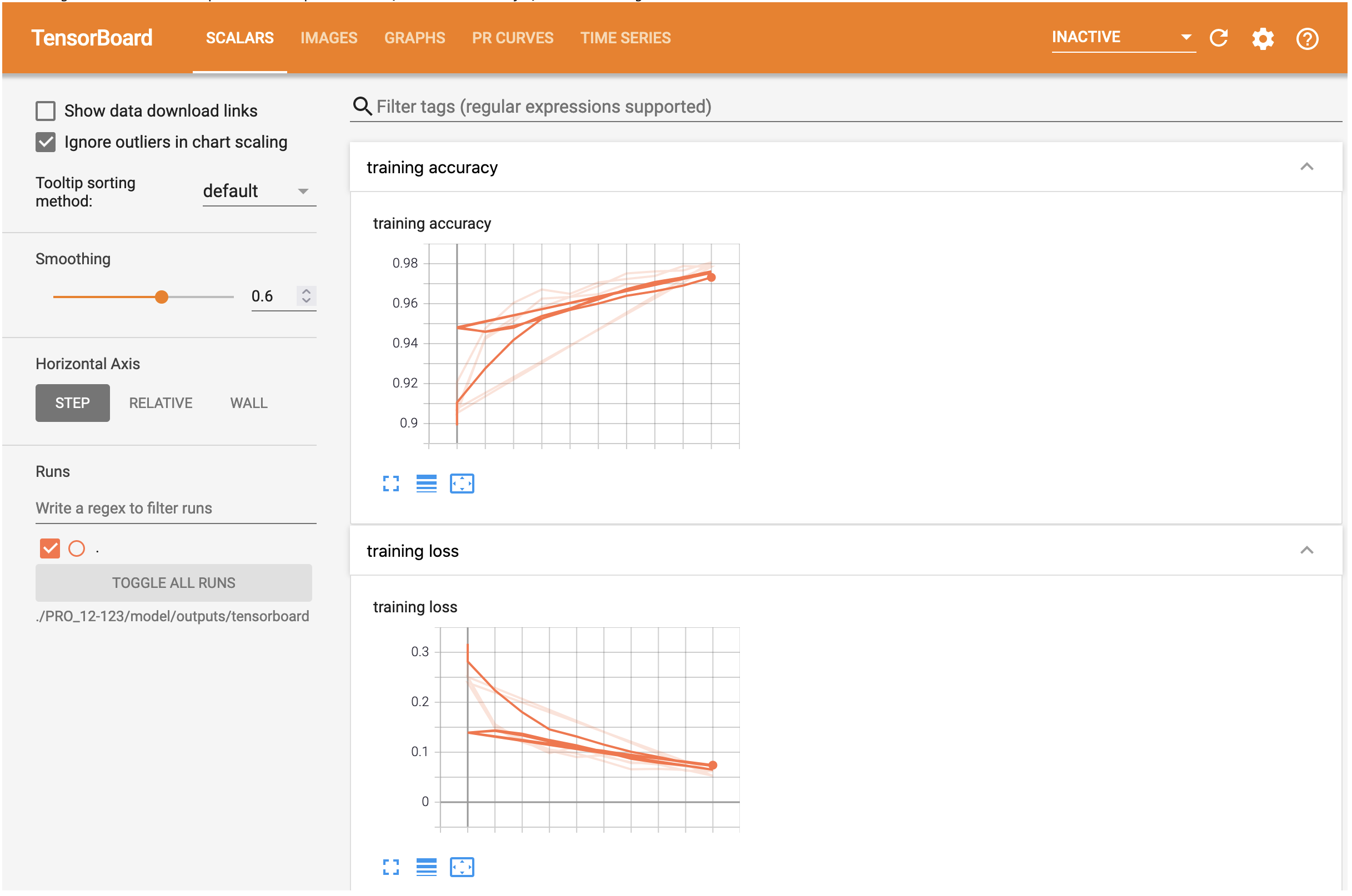
TensorBoard can generate figures that describe the accuracies and failings of our model based on the output files that we directed to output_dir. To view these figures, we can run a simple command that points the log directory to our local destination. When you run the following code block, you should see a TensorBoard extension within this notebook.

The first page, under the header SCALARS, depicts the progression of our model’s accuracy and loss scalars as it trains on the data. We can expect the accuracy to rise almost logistically and the loss to tend to zero.

The second page, under the header IMAGES, shows the validation confusion matrix. Note that the model should have higher marks for the labels that were more abundant in the training set, namely the tumors and arteries. Since the model is trained on so little data, do not be surprised if the confusion matrix differs quite drastically from the identity matrix.

The remaining pages will depict additional figures for our model, including a diagram relating our input and output to the model (residual neural network). Feel free to spend time exploring this extension!

tensorboard --logdir=./PRO_12-123/model/outputs/tensorboard --bind_all

Reusing TensorBoard on port 6011 (pid 63424), started 9 days, 17:53:38 ago. (Use '!kill 63424' to kill it.)

At this point, you have completed this notebook. Congratulations! You have successfully trained a deep learning model on your toy dataset! You are now ready to continue to the inference stage of the pipeline. Please navigate to the inference-and-visualization notebook.

previous

Tile Generation Tutorial

next

Inference and Visualization Tutorial